Pen Plotter Art & Algorithms, Part 2

^{— This post is a continuation of Pen Plotter Art & Algorithms, Part 1.}

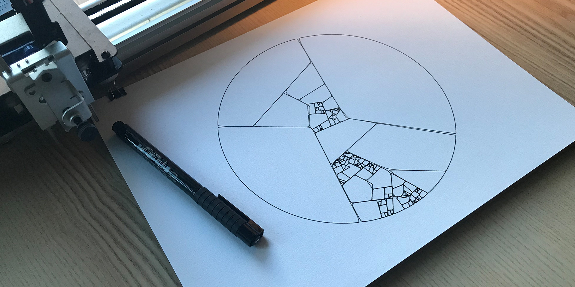
^{— Patchwork, printed with AxiDraw, December 2017}

In our previous post, we learned to develop some basic prints with penplot, an experimental tool I’m building for my own pen plotter artwork.

In this post, let’s aim for something more challenging, and attempt to develop an algorithm from the ground up. I’m calling this algorithm “Patchwork,” although I won’t claim to have invented it. I’m sure many before me have discovered the same algorithm.

💡 You can find more discussion and images in this Twitter thread, where I first posted about it.

The algorithm we will try to implement works like so:

1. Start with a set of N initial points.
2. Select a cluster of points and draw the convex hull that surrounds all of them.
3. Remove the points contained by the convex hull from our data set.
4. Repeat the process from step 2.

The “convex hull” is a convex polygon that encapsulates a set of points; it’s a bit like if we hammered nails down at each point, and then tied a string around them to create a closed shape.

To select a cluster, we will use k-means to partition the data into N clusters, and then select whichever cluster has the least amount of points. There are likely many ways you can randomly select clusters, perhaps more optimally than with k-means.

Initial Setup #

Install the required libraries first, and then generate a new script with penplot.

# install dependencies
npm install density-clustering convex-hull

# generate a new plot
penplot patchwork.js --write --open

Now, let’s begin by adding the same random points code from Part 1 and stubbing out an update function for our algorithm. We also need to return { animate: true }, so that penplot will start a render loop instead of just drawing one frame.

// ...

import { PaperSize, Orientation } from 'penplot';
import { randomFloat } from 'penplot/util/random';
import newArray from 'new-array';
import clustering from 'density-clustering';
import convexHull from 'convex-hull';

export const orientation = Orientation.LANDSCAPE;
export const dimensions = PaperSize.SQUARE_POSTER;

export default function createPlot (context, dimensions) {
  const [ width, height ] = dimensions;

  // A large point count will produce more defined results
  const pointCount = 500;
  let points = newArray(pointCount).map(() => {
    const margin = 2;
    return [
      randomFloat(margin, width - margin),
      randomFloat(margin, height - margin)
    ];
  });

  // We will add to this over time
  const lines = [];

  // The N value for k-means clustering
  // Lower values will produce bigger chunks
  const clusterCount = 3;

  // Run our generative algorithm at 30 FPS
  setInterval(update, 1000 / 30);

  return {
    draw,
    print,
    background: 'white',
    animate: true // start a render loop
  };

  function update () {
    // Our generative algorithm...
  }

  // ... draw / print functions ...
}

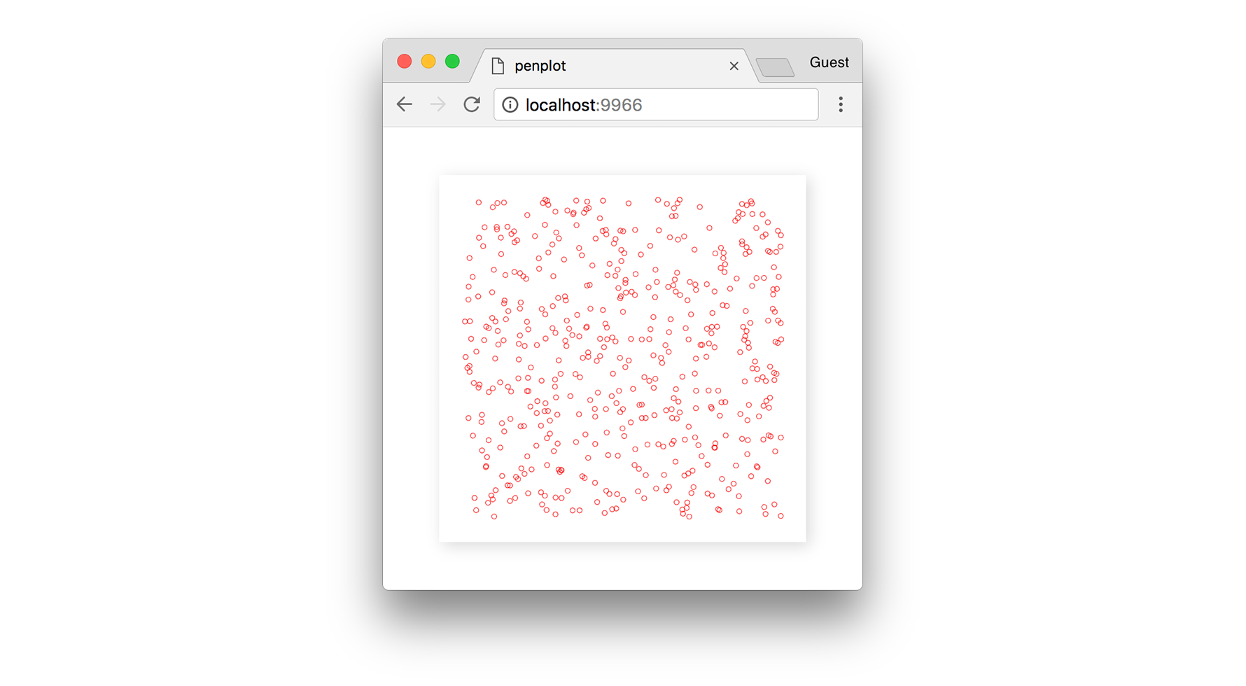
You won’t see anything yet if you run the code, that’s because our lines array is empty. If we were to visualize our random points, they would look like this:

Generating New Polygons #

Let’s make it so that each time update runs, it adds a new polygon to the lines array. The second step in our algorithm is to select a cluster of points from our data set. For this we will use the density-clustering module, filtering the results to ensure we select a cluster with at least 3 points. Then, we sort by ascending density to select the cluster with the least number of points (i.e. the first).

Like with triangulate(), the density clustering returns lists of indices, not points, so we need to map the indices to their corresponding positions.

function update () {
  // Not enough points in our data set
  if (points.length <= clusterCount) return;

  // k-means cluster our data
  const scan = new clustering.KMEANS();
  const clusters = scan.run(points, clusterCount)
    .filter(c => c.length >= 3);

  // Ensure we resulted in some clusters
  if (clusters.length === 0) return;

  // Sort clusters by density
  clusters.sort((a, b) => a.length - b.length);

  // Select the least dense cluster
  const cluster = clusters[0];
  const positions = cluster.map(i => points[i]);

  // ...
}

Now that we have a cluster, we can find the convex hull of its points, and removes those points from our original data set. The convex-hull module returns a list of edges (i.e. line segments), and by taking the first vertex in each edge, we can form a closed polyline (polygon) for that cluster.

function update () {
  // Select a cluster
  // ...

  // Find the hull of the cluster
  const edges = convexHull(positions);

  // Ensure the hull is large enough
  if (edges.length <= 2) return;

  // Create a closed polyline from the hull
  let path = edges.map(c => positions[c[0]]);
  path.push(path[0]);

  // Add to total list of polylines
  lines.push(path);

  // Remove those points from our data set
  points = points.filter(p => !positions.includes(p));
}

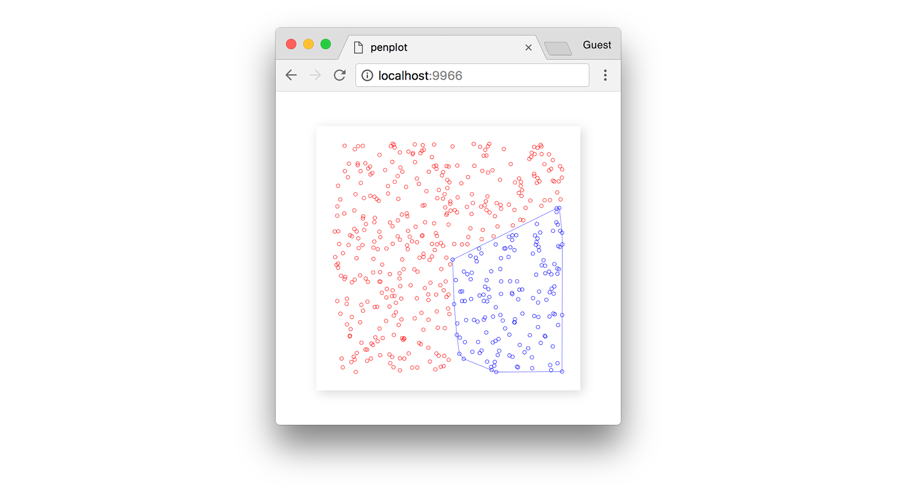
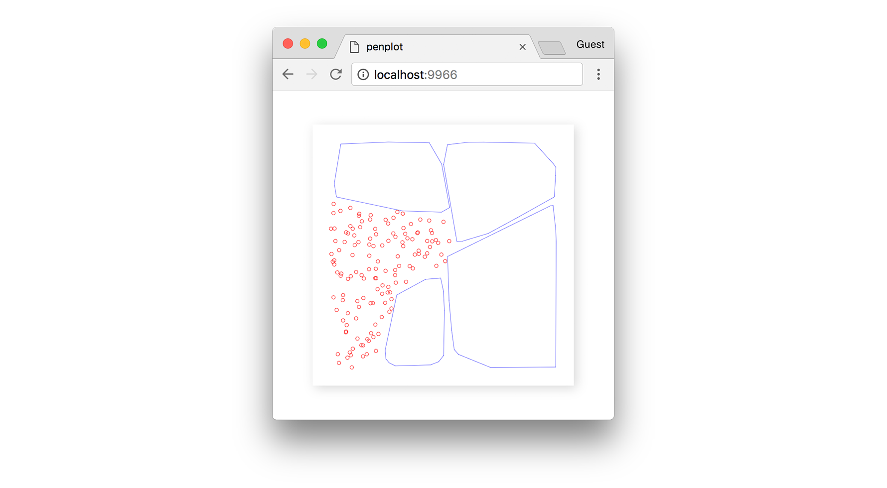
Below, we can see the set of blue points (a cluster) and their convex hull being defined around them.

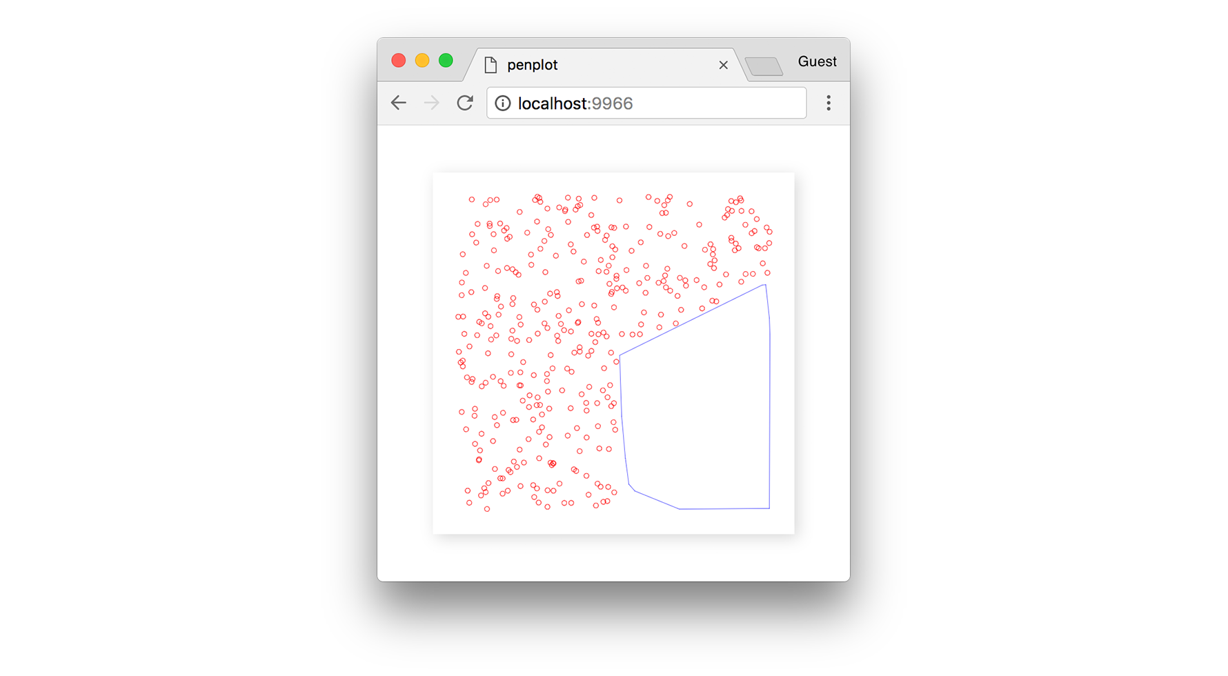
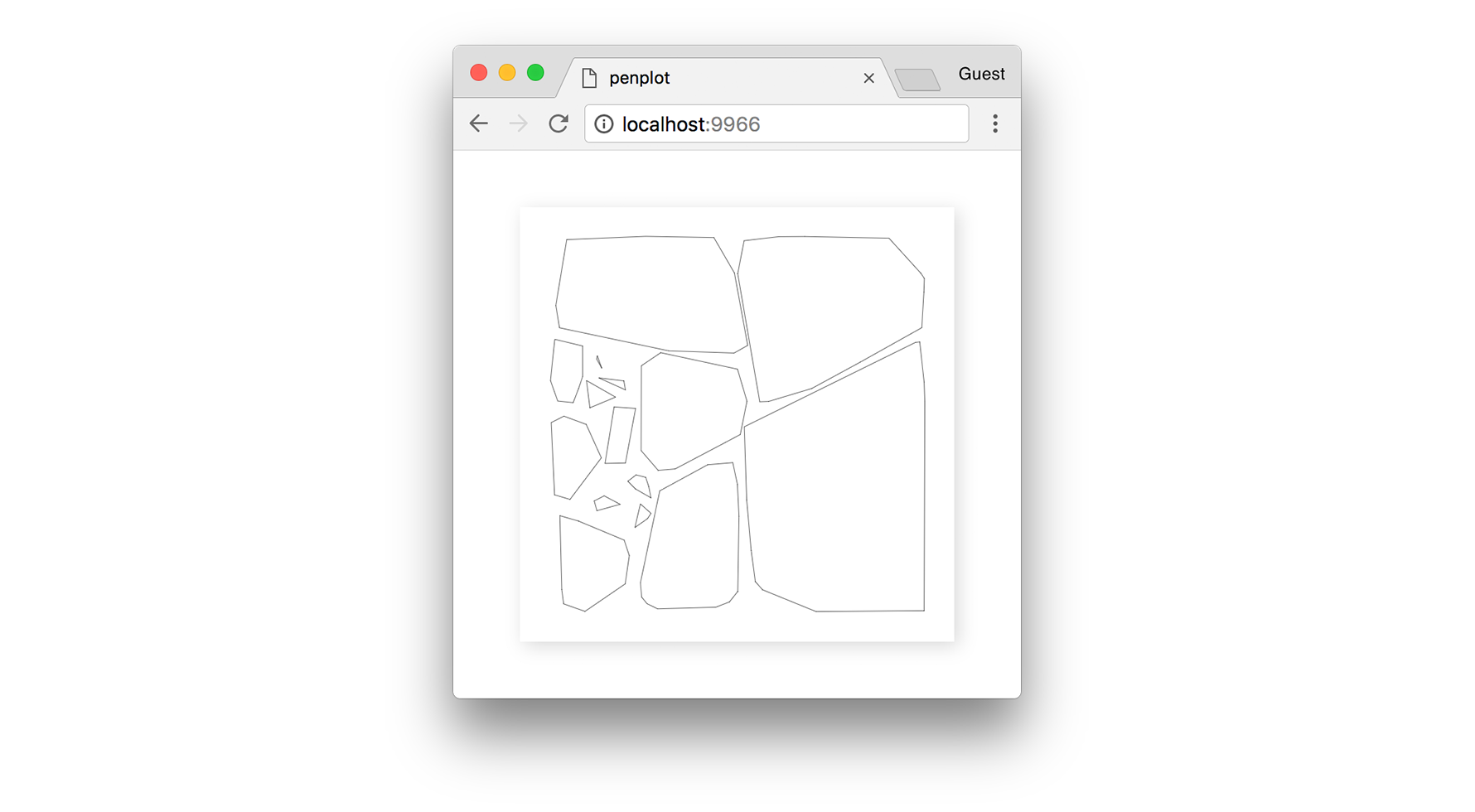
Once the points from that cluster are removed from the data set, we are left with a polygon in their place.

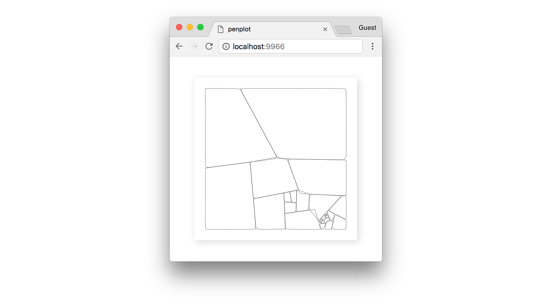
As we continue stepping the algorithm forward, we end up with more polygons filling in the empty space.

Until eventually the algorithm converges, and we can find no more suitable clusters.

Like in the triangulation example from Part 1, let’s increase our pointCount to get a more refined output. With a high number, like 50,000 points, we will get more detail and smoother polygons.

^{✏️ See here for the final source code of this print.}

Recursion #

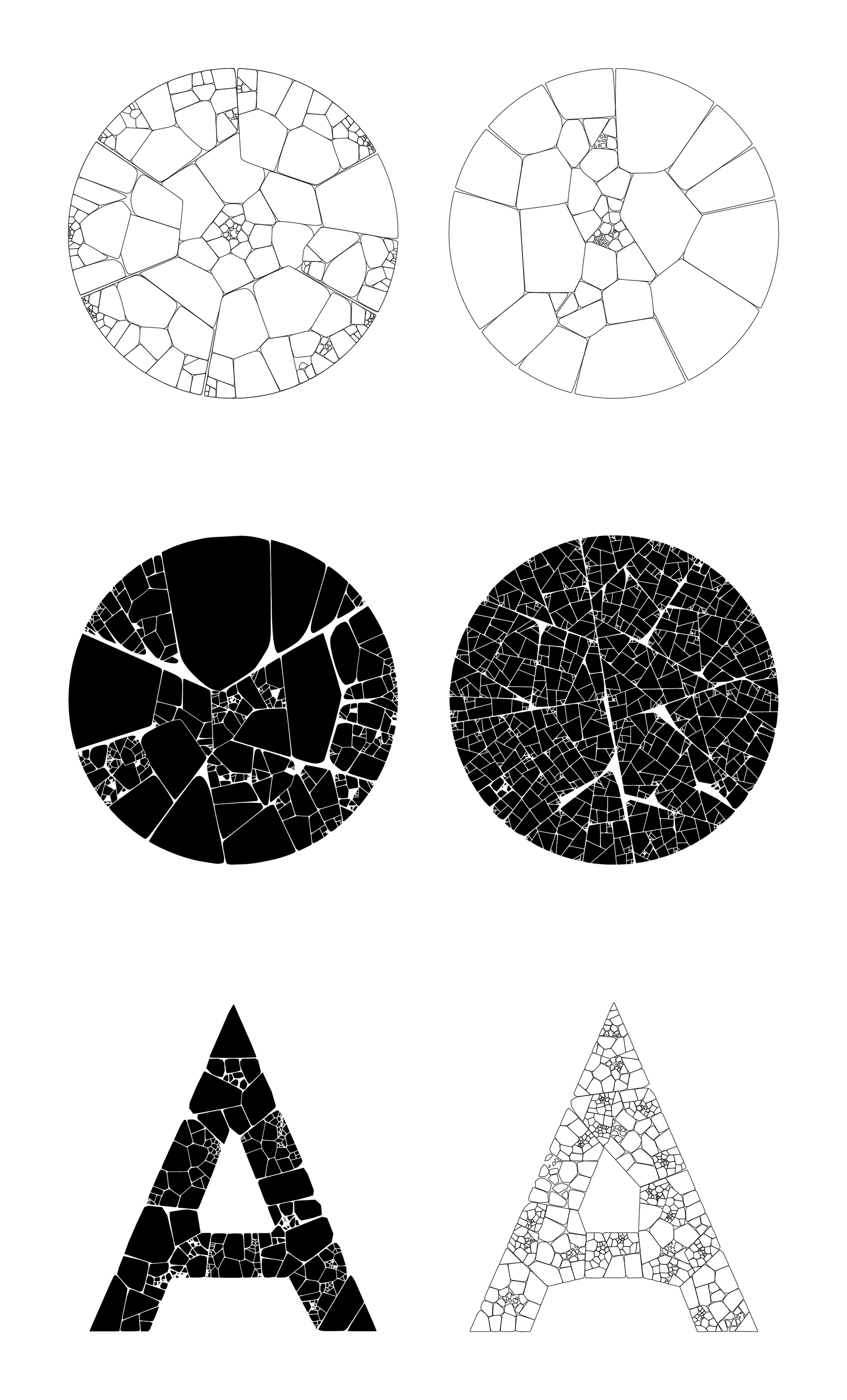
The real elegance in this algorithm comes from recursing it; after it converges, you can select a new polygon, fill it with points, and re-run the algorithm again from step 2. After many iterations, you end up with incredibly detailed patterns.

Below are a few other examples after spending an evening refining and tweaking a recursive version of this algorithm. These particular outputs use Canvas2D fill(), thus aren’t suitable for a pen plotter.

^{— Patchwork, December 2017}

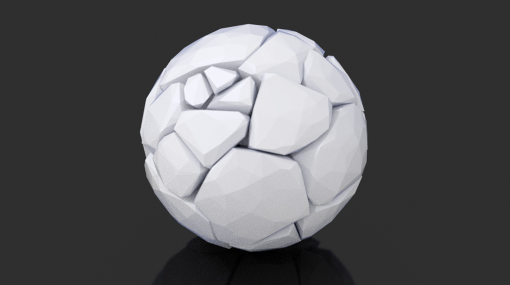
Other Applications #

It’s worth noting that the “Patchwork” algorithm can also be extend to 3D. The below model was exported from ThreeJS and rendered in Blender.

Since my original tweet, others have also implemented this algorithm in Houdini: see @cargoneblina, @sugiggy and @yone80.

Thinking Physically #

The biggest takeaway from learning to use a pen plotter is how I am starting to think in more physical terms — even something as simple as using centimetre units instead of pixels.

As you can see from the earlier 3D render, this algorithmic pen plotter work is naturally leading me to other physical outputs with JavaScript. In a future post, I hope to detail my workflow for parametric 3D modelling in ThreeJS to create foldable paper models, laser cut artwork, and more.

Further Reading #

If you enjoyed this blog post, you should take a look at some other artists working with pen plotters and generative code.

• Anders Hoff (Inconvergent) writes a lot about his process in Python and Lisp.
• Michael Fogleman wrote a blog article on pen plotter basics. He’s also written tools like ln, a 3D to 2D line art engine for Go.
• Tyler Hobbs writes about generative art and programming, and his work shares many parallels with my process here.
• Paul Butler recently wrote a blog post on his pen plotter work in Python.
• Tobias Toft explains how to use Processing with traditional HP plotters. These use a different file format, but are often more affordable than the AxiDraw.

You can find lots more pen plotter work through the Twitter hashtag, #plottertwitter.